Basic Usage
The central object in the LRSplines-package is the LRSpline object. We initialize an LRSpline at the tensor-product level by specifying two knot vectors, and corresponding polynomial degrees. The following code initializes a biquadratic LR-spline.
Initialization and mesh visualization
import LRSplines

du = 2
dv = 2
knots_u = [0, 0, 0, 1, 2, 3, 3, 3]
knots_v = [0, 0, 0, 1, 2, 3, 3, 3]

LR = LRSplines.init_tensor_product_LR_spline(du, dv, knots_u, knots_v)
We can at any stage visualize the LR-mesh which underlies a given LR-spline, as seen:
LR.visualize_mesh()
yielding the image
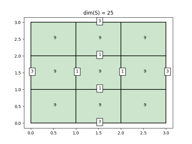
Here, each element of the mesh displays the number of supported B-splines. In this case there are nine supported B-splines on each element. The green color indicates that the element is not overloaded. Each meshline displays its multiplicity indicated by a number in a white box. As we can see, the boundary mesh-lines have multiplicity 3, which reflects the knot vectors we chose. The dimension of the spline space is displayed at the top. In this case, we have five basis splines in each direction, totaling 25 tensor product B-splines.
Meshline insertion
We can insert mesh-lines into the mesh by creating a new Meshline object. In this example, we insert a meshline between the points (1.5, 0) and (1.5, 2) and between the points(1, 1.5) and (3, 1.5). This is represented in Python as:
m1 = LRSplines.Meshline(start=0, stop=2, constant_value=1.5, axis=0)
m2 = LRSplines.Meshline(start=1, stop=3, constant_value=1.5, axis=1)
The axis parameter determines the direction of the meshline, i.e., 0
for vertical and 1 for horizontal. We insert this meshline into the
LR-spline, and visualize the result.
LR.insert_line(m1)
LR.insert_line(m2)
LR.visualize_mesh()
This yields the following image:
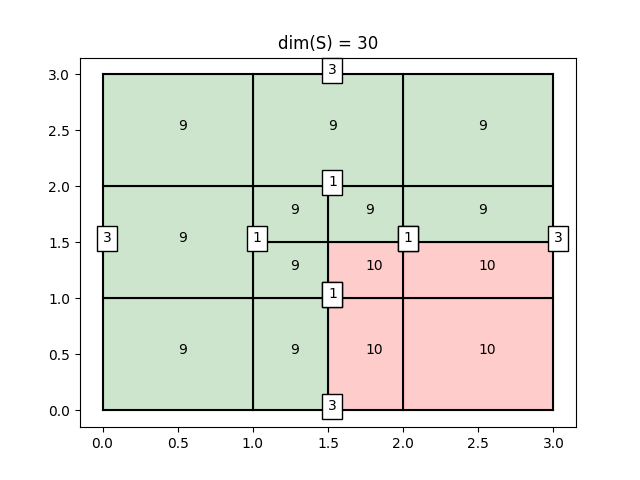
As we can see, some of the elements have turned red, indicating that they are now overloaded, which may result in loss of linear independence.
Evaluation
We can at any stage evaluate the LR-spline. At the moment there is no
clever functionality for setting the coefficients of the underlying
B-splines, but we can do so explicitly by looping over the set of basis
functions LR.S.
import numpy as np
import matplotlib.pyplot as plt
from mpl_toolkits.mplot3d import Axes3D
# set the coefficients explicitly
for b in LR.B:
b.coefficient = np.random.random(-3, 3)
N = 20
x = np.linspace(knots_u[0], knots_u[-1], N)
y = np.linspace(knots_v[0], knots_v[-1], N)
z = np.zeros((N, N))
X, Y = np.meshgrid(x, y)
for i in range(N):
for j in range(N):
z[i, j] = LR(x[i], y[j])
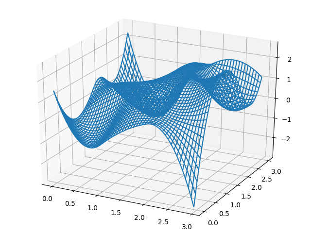
fig = plt.figure()
axs = Axes3D(fig)
axs.plot_wireframe(X, Y, z) # or plot_surface
This gives the resulting surface: